4.2. The postprocessor

The PostProcessor-class is responsible for all the logic behind the scenes. This includes logic related to:

• Dependency handling
• Planning and caching of computation
• Saving
• Plotting

The planning, saving and plotting is delegated to dedicated classes (Planner, Saver and Plotter), but is called from within a PostProcessor-instance.

4.2.1. The update_all-function

The main interface to the user is through the PostProcessor.update_all()-method. This takes three arguments: a dict representing the solution, the solution time and the solution timestep.

The time and timestep is used for saving logic, and stored in a play log and metadata of the saved data. This is necessary for the replay and restart functionality, as well as order both the saved and plotted fields.

The solution argument should be of the format:

solution = dict(
    "Velocity": lambda: u
    "Pressure": lambda: p
)

Note that we pass a lambda function as values in the dict. This is done to give the user the flexibility for special solvers, and can be replaced with any callable to do for example a conversion. This can be useful when there are discrepancies between the solver solution, and the desired physical solution. This could be for example a simple scaling, or it could be that a mixed or segregated approach is used in the solver.

Because this function might be non-negligible in cost, it will be treated in the same manner as the Field.compute()-method, and not called unless required.

4.2.2. Dependency handling

When a field is added to the postprocessor, a dependency tree is built. These dependencies represent the required fields (or time parameters) required to succesfully execute the compute-method.

The source code of the compute-function is inspected with the inspect-module, by looking for calls through the get-argument, and build a dependency tree from that.

Assume that the following code is executed:

pp = PostProcessor()
pp.add_field(SolutionField("F"))
pp.add_field(TimeDerivative("F"))

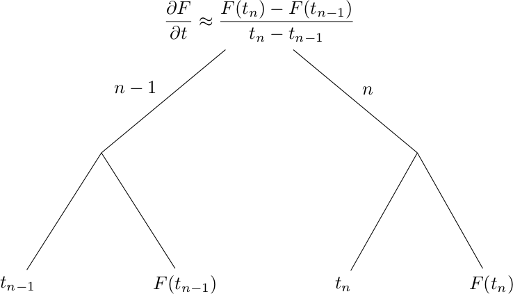
In that case, when the TimeDerivative-field is added to the postprocessor, the following code is inspected:

class TimeDerivative(MetaField):
    def compute(self, get):
        u1 = get(self.valuename)
        u0 = get(self.valuename, -1)

        t1 = get("t")
        t0 = get("t", -1)

        # ... [snip] ...

By evaluating the get-calls here, we are able to build the following dependency tree:

If we extend the above example to add the time derivative of the viscous stress tensor (see A viscous stress tensor) like the following:

pp = PostProcessor()
pp.add_fields([SolutionField("Velocity"), SolutionField("Pressure")])
pp.add_field(Stress())
pp.add_field(TimeDerivative("Stress"))

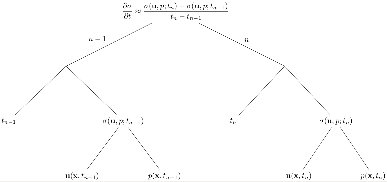
The first emphasized line will trigger building of the dependency tree for the stress:

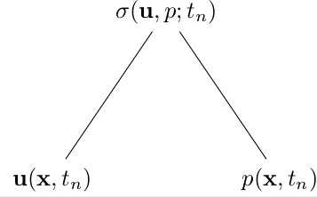
while the second emphasized line will use this dependency tree, and trigger the building of the larger dependency tree

4.2.3. Planner

The Planner-class will set up a plan of the computations for the coming timesteps. This algorithm will inspect the dependencies of each field, and compute the necessary fields at the required time.

In addition, it determines how long each computation should be kept in cache.

Note

This does not yet support variable timestepping.

4.2.4. Saver

The Saver-class handles all the saving operations in cbcpost. It will determine if and how to save based on Field-parameters. In addition, there are helper methods in PostProcessor for saving mesh and parameters.

For fields, several saveformats are available:

Replay/restart-compatible	Visualization	Plain text
hdf5	xdmf	txt
xml	pvd
xml.gz
shelve

The default save formats are:

• hdf5 and xdmf if data is dolfin.Function
• txt and shelve if data is float, int, list, tuple or dict

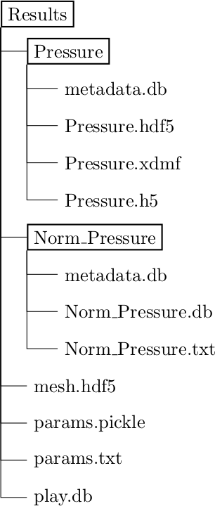
The saving is done in a structured manner below the postprocessors case director. Consider the following example:

pp = PostProcessor(dict(casedir="Results/"))
pp.add_fields([
    SolutionField("Pressure", save=True),
    Norm("Pressure", save=True),
])
pp.store_mesh(mesh, facet_domains=my_facet_domains,
              cell_domains=my_cell_domains)
pp.store_params(
    ParamDict(
        mu = 1.5,
        case = "A",
        bc = "p(0)=1",
    )
)

Here, we ask the postprocessor to save the Pressure and the (L2-)norm of the pressure, we store the mesh with associated cell- and facet domains, and we save some (arbitrary) parameters. (Note the use of ParamDict).

This will result in the following structure of the Results-folder:

4.2.5. Plotter

Two types of data are supported for plotting:

• dolfin.Function-type objects
• Scalars (int, float, etc)

The Plotter-class plots using dolfin.plot or pyplot.plot depending on the input data. The plotting is updated each timestep the Field is directly triggered for recomputation, and rescaled if necessary. For dolfin plotting, arguments can be passed to the dolfin.plot-command through the parameter plot_args.

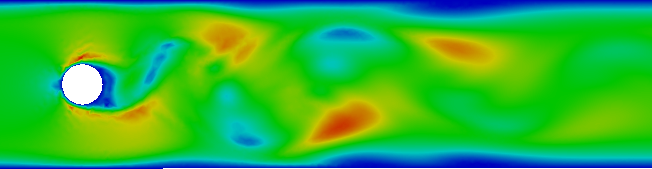
dolfin.Function objects are plotted with dolfin.plot

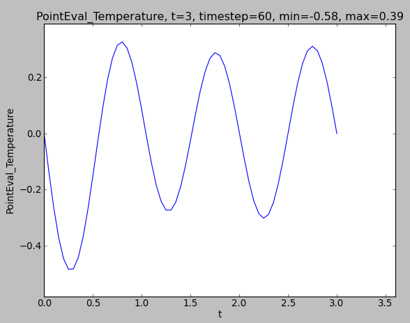
Simple scalars are plotted with pyplot